New perspective for Overfitting and Underfitting -- Bias and Variance Decomposition
You probably all heard of overfitting and underfitting. You might also heard of Occam’s razor, which is borrowed from philosophy as a preference for simpler model than complex model in machine learning to avoid overfitting. However, these concepts either sound too empirical or too philosophical. Bias and Variance decomposition is a mathemetical approach for the analysis of this problem. So how does it work? Let’s get an intuitive understanding of it by looking at the polynomial regression problem.

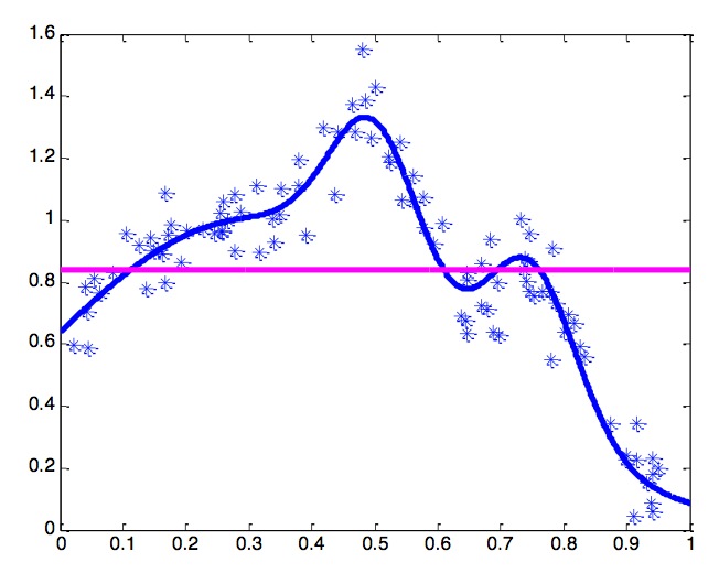
The blue curve is a polinomial curve with k=5, representing a data distribution. The blue “*”s are points sampled from the distribution with a gaussian noise. And if we use linear regression to fit these data points we will get the red line.
If there’re multiple datasets sampled from the same data distribution, then we might expect such results from fitting a linear model:

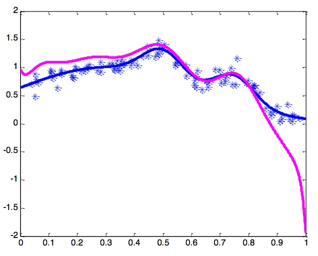
On the other hand, if we use a k larger than 5 (say, 7), we might fit a curve like this:

Again, given multiple datasets from the same distribution, we might get this for the same k:

From these figures we can see that the linear model is deviated from the data points a lot, but the results we get from different sampled data are very similar; on the other hand, a polynomial curve with a large k might fit the data points quite well, but each time we run it on a different sampled of the same distribution we might get a very different result.
That’s the basic intuition of Bias-Variance decomposition(or Bias-Variance Tradeoff). We say that linear model has large bias but small variance, while the large-k-polinomial model has small bias but small variance. By doing some maths, it shows that on average, this two terms add up to the error of our model on average. This means if either of bias and variance is big, we are probably not getting a satisfying model.
Here comes the math
Now let’s use Y to represent the true value of all points, to represent the underlying data distribution model we can get (since there’re noises so it’s different from Y). And f(x) is the model we fit. The first step of Bias-Variance decomposition tells us:
The term on the left of the equation means how much the model we fit is different from the observed values of data points on average. It turns out to be the summation of two terms: how much the model we fit is different from the underlying model, and how much the observed values differ from the data distribution(again, because of noises).
The next paragraph is the proof. If not interested can skip it:
Proof:
And
So we have
The term is beyond our reach, since we can do nothing about it, so let’s focus on what we can do: we can further decompose the term .
Let’s just skip to the conclusion(the proof is similar to the previous one):
Dn is the dataset we use. Let’s take a look at the two terms on the right side of the equation. The first term measures the variance of the models we get each time(Variance), the second term measures that on average, how far our models are from the groundtruth(Bias).
Now let’s see how can this guide us through machine learning practise. Bias is how well the model approximates the groundtruth(represented by the observed data). A simpler model (linear model in the previous example) will have larger bias. When the bias is always too big, then the model is underfitting, which means it doesn’t have enough flexibility to capture the right model. On the other hand, when we choose a model that’s too flexible, it may be fitting the data points very well, but a small change of the dataset could produce a completely different model, so the variance would be large. Neither is good. In practise, we should try to find a balance. The figure below could better illustrate the idea:

Similar figures might also be used to illustrate the idea of overfitting. From my perpectives, it’s just a different way to represent the same idea.
Summary: Bias-Variance is a mathematical way to understand what underfitting and overfitting mean. In practise we should find a balance point to avoid either bias or vairance being too large.
Reference: Figures and initial equations come from the the lecture slides of Prof. Singh in Carnegie Mellon University.